Document 104
Evaluation of Scientific Notebook 3.5 as a Tool in Mathematics Education
Mirek Majewski
Department of Mathematics and Computer Science, Inter-University Institute of Macau, NAPE, Lote 18, Rua de Londres - P, Edf. Tak Plaza, R/C - 3, MACAU
Email: mirekmajewski@yahoo.com
Abstract
Teachers of mathematics all over the world are searching for teaching tools that can improve the teaching process, i.e. make it attractive for students, let them visualize most of the mathematical concepts, free students from tedious calculations and mechanical errors giving them an opportunity to concentrate on the algorithms and methods of solutions. In this paper I examine a computer program called Scientific Notebook 3.5 and I show how useful it can be in high school mathematics, university mathematics and engineering education.
1. Introduction
Scientific Notebook 3.5 is a relatively new product from TCI Software Research (now MacKichan Software, Inc.). It is a simplified version of their Scientific WorkPlace and an adapted extension of their Scientific Word. Both programs are valuable and widely accepted tools in mathematical research and DTP involving mathematical and technical documents.
Scientific Notebook 3.5 has three basic components: a word processor, a computation engine that is a Maple kernel, and an exam builder. The three components form a very interesting environment for working with mathematics. First I will describe some features of Scientific Notebook's word processor that are important for editing mathematical and technical documents. Later I shall concentrate on the mathematical properties of Scientific Notebook and I show a few selected examples of mathematical problems and their solutions. Finally I will show how Scientific Notebook can be useful in communication between students and teacher, and also in distance education.
2. The Word Processor
Three features of the Scientific Notebook 3.5 word processing capabilities are very important for the user, namely its
-
general word processing functions
-
formula editor
-
hypertext generating functions.
2.1. General word processing functions
Scientific Notebook 3.5 uses a slightly different approach to word processing than most of its contemporary editors. On first look, its screen formatting functions seem to be a bit limited, however later we will discover that it has everything that we need. In most word processors the user has freedom of formatting on the screen, i.e. changing fonts, their size etc. This leads to the situation, that while having perfect word processing tools, we still use them in the same way like old typewriters. We manually do most of the formatting functions; we manually change the size of letters in headers; we add empty lines between paragraphs; we manually insert page breaks and sometimes even line breaks, etc. These are old and bad habits which are not easy to change. Scientific Notebook forces us to do logical, rather than physical, formatting of the text. First, when we start a new document, we start it by choosing a specific shell with a number of predefined tags. Here 'shell' has the meaning of the word 'template' as used with other word processors, while 'tag' means style.
There are a number of shells that are very convenient for editing mathematical documents, scientific articles, exams and tests, laboratory reports, on line mathematics, etc. Of course we still have the possibility of defining our own shells and in Scientific Notebook this is a rather easy task. In Scientific Notebook we do not have control of how lines of the text will be formatted in the printout, i.e. which word will be last in the line and where a page will end. We see on the screen as much of the text as can fit in the window. Text is wrapped relative to the size of the window not to the page size. This approach is typical for all TEX based text formatting tools. Type your text, emphasizing some parts of the document using the appropriate tag (body tag, header tag, or any other), concentrate on the contents, and the rest will be done for you in the best possible style. It is even possible to configure Scientific Notebook in that way that all multiple spaces or eoln markers will be reduced to a singe space or a single eoln marker.
Scientific Notebook 3.5 writes its files in TEX format. This is the widely accepted format for mathematical and technical documents. Printing is done throughout standard Windows 95 drivers and true type fonts, which gives us a bit more flexibility than printing from LaTeX. However text saved in Scientific Notebook can be compiled and printed by most of the TEX compilers.
2.2. Formula Editor
Most of the contemporary word processors have some utilities for producing mathematical formulae. One of the most developed and the most popular is the Microsoft Equation Editor. Using this tool we produce a formula and embed it into any MS Word document. We can also embed any MS equation into any file if the program generating this file supports Microsoft object linking and embedding technology. This is the way we add formulae to Excel spreadsheets, Page Maker, Ventura documents, etc. Unfortunately in each case the formula is an alien body in that document. A consequence of this fact is that documents with such formulae are very large and editing them is sometimes a very annoying process. Try to edit a document with hundreds of formulae in any word processor using this approach.
In Scientific Notebook 3.5 mathematical formulae are integral parts of the document. All Scientific Notebook documents are stored in TEX format as well as all formulae. This means that a formula sin(x) and the word sin(x) are coded inside of the document, however a formula is treated a bit differently than a word with the same appearance. We use two modes -- one for text editing, and one for formula editing. To switch between both modes we use the [Ctrl-M] command or appropriate icon on the screen. Scientific Notebook recognizes formulae that are typed in maths mode and formats them according to the international typographic rules. Most of the formulae we are dealing with are multi-leveled objects with subscripts, superscripts, fractions, limits, etc. We can enter them using keyboard shortcuts (my preferred way) or by choosing them from some toolboxes or menus. Using keyboard shortcuts is the most convenient way of editing mathematical formulae. It is so comfortable that after using Scientific Notebook you will be not satisfied with any other word processor.
There are a large number of structural operators and mathematical symbols that we can use in Scientific Notebook. Figures 3 and 4 show some examples. Libraries of symbols used by Scientific Notebook cover probably all symbols that have been used by mathematicians throughout centuries. I found large sets of binary operators and relation symbols as well as special characters and arrows used for creating various diagrams.
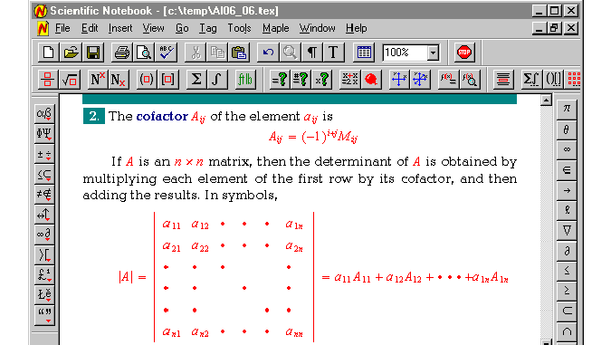
Figure 1. Scientific Notebook is a perfect tool for editing
mathematical
documents
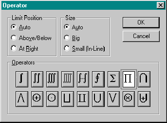
Figure 2. Scientific Notebook's operator toolbox--we can choose an operator, position of subscripts, superscripts and their size.
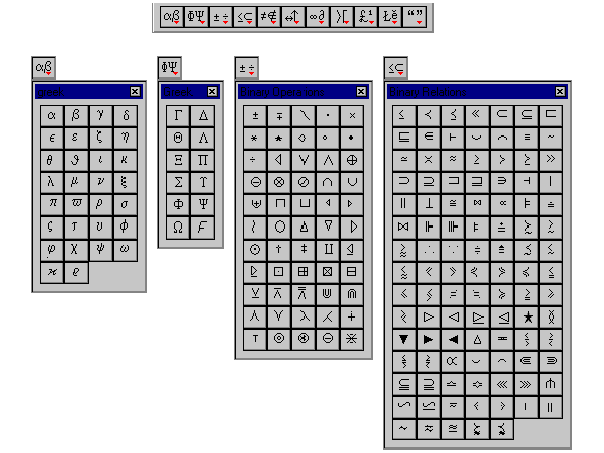
Figure
3. Selected libraries of symbols that are implemented in Scientific
Notebook.
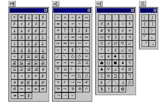
Figure
3a. Selected libraries of symbols that are implemented in Scientific
Notebook.
Scientific Notebook 3.5 recognizes many mathematical functions as well as functions defined by the user. We can define a function while working with Scientific Notebook, save this function with a document and use it in the future. The class of predefined functions supported by Scientific Notebook is very large and covers probably most of the standard functions known in mathematics. All functions recognized by the program appear on the screen as a gray text. If the function, you typed in maths mode, doesn't appear as a gray text it means the spelling of the name of the function is wrong. In such case we can choose the name of the function from a large list of predefined functions. The name of any user-defined function can also be added to the extensive library of function names.
3. Doing Mathematics with Scientific Notebook
As stated earlier, the computing engine in Scientific Notebook 3.5 is a Maple V R4 kernel. Scientific Notebook 3.5 serves as a convenient interface for Maple. We do not need to know a large number Maple commands and functions, most of them are accessible directly from Scientific Notebook 3.5 menu or by key shortcuts. For instance, to evaluate an expression we do not need to remember a Maple eval command, we can choose it from the appropriate menu, or press [Ctrl-E], or press the Evaluate button. This method is much more convenient if we use standard Maple operations. If we are working with more sophisticated mathematics, sometimes we have to call a Maple function directly, but this is not a very complicated process. The Maple kernel inside of Scientific Notebook 3.5 is a bit limited---some Maple functions and operations are missing. If we have a Maple V R4 original kernel, we can connect Scientific Notebook 3.5 to it without any problem. In this way we can extend the functionality of the Scientific Notebook.
One of the most interesting features of Scientific Notebook 3.5 is the opportunity to use external user-defined functions. Such functions should be written in the Maple language and saved in Maple as a Maple library, i.e. the file *.m. This very powerful feature of Scientific Notebook enables us to use almost unlimited number of functions and relations. This, however, is not a very straightforward process and unfortunately not all user-defined functions work correctly in Scientific Notebook.
Scientific Notebook 3.5 can be used in two different ways. One way, often
called the black box method, can be very useful in situations where the
emphasis is on the initial problem and a final solution. Scientific Notebook
3.5 has implemented a large library of mathematical operations like solving
equations, differentiation, integration, etc. This means that for many
problems, but perhaps not for all, it is enough to properly identify a problem
and to choose an appropriate method from the Maple menu. Here you can find a
number of operations: evaluate an expression, evaluate numerically, simplify,
combine, factor, check equality, various operations on polynomials, calculus,
power series, solving differential equations, operations on matrices, plotting
in 2D and 3D
etc.
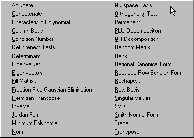
Figure 4. The Scientific Notebook 3.5 Maple menus offer a number of mathematical operations, here is shown the Matrix menu.
Another way of solving problems goes through showing all immediate steps from formulated problems up to a final solution. This method is a very powerful instrument in mathematics education and experimenting with various methods of solving mathematical problems. Teachers explain each step of solution by showing how Scientific Notebook transforms an initial formula.
One of the most interesting features of Scientific Notebook 3.5 is the ability
of performing some operations in place or locally. It is enough to select a
part of the mathematical expression and choose the appropriate operation that
should be performed locally. For example having a formula:
 we can select only
 and choose operation Expand (with the Ctrl key down). The initial formula will
be transformed to the form where only the first term will be expanded. The
second term will remain in its original form. Performing an operation in place
is a unique feature of Scientific Notebook that is not available in other
mathematical packages.
and choose operation Expand (with the Ctrl key down). The initial formula will
be transformed to the form where only the first term will be expanded. The
second term will remain in its original form. Performing an operation in place
is a unique feature of Scientific Notebook that is not available in other
mathematical packages.
I include here three short examples. I am sure that these examples do not show all the interesting features of Scientific Notebook 3.5, however I have included them to demonstrate a general idea of how we can work with Scientific Notebook. If you need more information, you can find it easily. On the CD with Scientific Notebook are included large help files with essential information on how to use this program in various mathematical disciplines. Scientific Notebook help files provide you not only with information on how to use this program, but also enables you to find comprehensive information about hundreds of mathematical terms and topics. On the CD there is also enclosed a large textbook Doing Calculus with Scientific Notebook, by Darel W. Hardy and Carol L. Walker.
All information enclosed with Scientific Notebook is in TEX format. If you are like me, and you like reading in bed, you can print any file and read it just before going to sleep. I can assure you that this is very interesting reading.
4. Exam and test builder
If you are a teacher of mathematics or physics you will appreciate the Exam Builder. This part of Scientific Notebook 3.5 can save you a lot of time both in preparing exams and tests, as well as in marking them.
Exam builder can be used to generate various kinds of exams, tests, assignments, quizzes, tutorials or simply training materials for our students. Such materials can be printed or simply left online on the computer network or Internet.
Preparation of such material is fairly simple. Our main task is to write a Scientific Notebook document with questions and solutions. In this document we declare variables of various types, define the range for them and ask Scientific Notebook to generate random data for these variables. For example we can use a random matrix of a given dimension with coefficients fulfilling some initial conditions. Most of the questions that can be done this way are multiple-choice questions, where the student has a choice of a few responses and he has to choose the proper one. Other types of questions we can generate are questions with some variants.
There are a few keywords that identify any part of such document: Comment, Text, Setup, Choices, Response, etc. The list of keywords is not very large, however we can find everything that we need here.
A file with a test or exam should be saved with extension .qiz. When the student opens such a file, Scientific Notebook uses keywords and algorithms included in the document to generate data for the test and displays it on the computer screen. Each time we open the same *.qiz file these data will be quite different as well as the order of questions and answers can be different. This means that each time the student deals with the same kind of questions, however, different data is always on the screen. After finishing such a test, Scientific Notebook can grade the students' results.
Tests done in Exam Builder provide very good drilling tools. The student can
open a test file as many times as he wishes and do it again and again up to
the moment when his mark will be acceptable for him. Figures 5 and 6 show two
different runs of the same test
file.
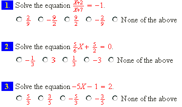
Figure 5. Test file equations.qiz in Scientific
Notebook
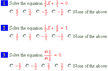
Figure 6. The same test again. Compare both pictures and observe how different are both tests.
5. Maple versus Scientific Notebook
As mentioned earlier, Scientific Notebook 3.5 uses a Maple kernel as a computing engine. One may think that both Maple and Scientific Notebook 3.5 have similar power and these programs are in some way equivalent. However, both programs are quite different not only in how they look on the computer screen, but also in how they work.
Scientific Notebook 3.5, due to its word processing functions, is a very convenient environment for writing documents and performing mathematical operations inside of them. Access to most of the mathematical operations and functions is very easy.
At the same time Maple has rather crude interface and to use it efficiently we have to know hundreds of Maple commands. For example to plot the parametric function
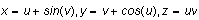
we use Maple commands:
>with(plots);
>plot3d([u+sin(v),v+cos(u),u*v],
>u=-2*Pi..2*Pi,v=-2*Pi..2*Pi, grid=[50,50]);
In Scientific Notebook 3.5 it is enough to type an equation of the function and to choose the appropriate operation from the Maple menu or simply press the Plot 3D Rectangular button.
Maple can be used to experiment with complicated computational processes. We type the contents of the Maple worksheet and run it to obtain results. When we change some of the conditions or functions used in our worksheet, we run the worksheet again and all results will be recalculated. These kind of operations are not possible in Scientific Notebook 3.5, however functions defined during Scientific Notebook sessions can be saved with a file and used again when the file is loaded next time. Graphs of functions are not saved in the file, these graphs are plotted each time Scientific Notebook loads the file.
6. Internet and Distance Education
While editing documents in Scientific Notebook 3.5 we can include in our text various kinds of links: link to a note or a hint, links to markers in a currently edited document or to any other document, links to files located on the Internet, or links to external programs. This means we can create large hypertext documents linked to all relevant resources available on the local computer and on the Internet. For instance a tutorial about the power series may include links to some basic topics like definition of a series, geometric and arithmetic series, basic properties of series, as well as links to much advanced information about functional series of complex functions. A student reading such documents will be able to choose the kind and level of information he needs.
We do not need to create all the documents which we link from our texts. We
can put a link to any other document available on the Internet. Of course it
is always a good policy to ask the author or owner of the document about
permission.
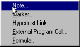
Figure 7. Various types of links we can insert into a Scientific Notebook document from the Insert menu.
Scientific Notebook 3.5 may be very useful in open and distance education. For this purpose we need a WWW server and Scientific Notebook together with MS Internet Explorer, installed on the local workstations.
Such WWW site may contain various documents in HTML or TEX format. For
instance we can put a set of tutorials there, with pictures, formulae,
diagrams, movies, sounds, etc. For each subject we can leave on the web server
lecture notes, as well as assignments, tests and exam for any subject. For the
students' convenience there should be one web page with a description of the
site and links to specific subjects. For instance the default web page may
list titles all subjects with links to web pages related to these subjects.
From this page we can jump to the pages with information related to a specific
subject. Here we may have links to separate tutorials, assignments, tests etc.
Such a web site may have a very simple tree-like structure. For example, as
shown in figure
8.
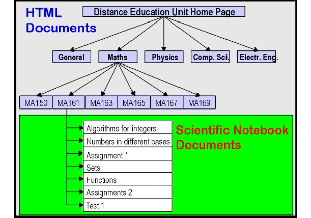
Figure 8. An example of a web site for Distance Education Unit. Scientific Notebook can be used here as a viewer of lecture and test files for each subject. Other documents are standard HTML pages.
Students, from any place in the country, at any time, using their home computers or computers in the local high school, can connect to this web site, read or print tutorials, do assignments, tests, or exams. Using Scientific Notebook 3.5 the student is able to communicate with his teachers. He can write a document with solutions of some problems, he can also formulate his own problems and send them to his teachers.
This kind of communication can be very fast and efficient. Scientific Notebook
3.5 cooperates with Internet Explorer very well. Each time we choose in
Scientific Notebook menu File-Open Location it opens it by means of Internet
Explorer. Each time we choose Send, it uses MS Exchange program to send
currently edited document throughout the local network or
Internet.
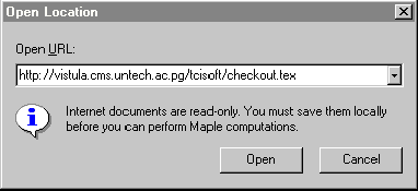
Figure 9. Scientific Notebook open location dialog box
7. Conclusions
I found Scientific Notebook 3.5 a very good instrument for teaching mathematics in high school, college and university. Application of Scientific Notebook 3.5 in some of the university subjects seems to be a bit limited, for example, the use of recursive functions, functions with iterations or implicit plots of 3D surfaces. In other mathematical disciplines Scientific Notebook 3.5 is the most desirable tool for both teaching staff as well as students.
Exam builder is a unique tool, that can enhance not only the testing or examination process but it can also be priceless in producing training materials for students.
Finally Scientific Notebook 3.5 as an Internet ready tool can be used not only locally but also beyond the local network. It can be used to access documents stored in TEX format on the Internet. Students, using their home computers, will be able to read Scientific Notebook documents left on the school WWW server. They can access documents with assignment questions, write solutions in Scientific Notebook and send their work by e-mail to the teacher for marking.
8. Appendix
The appendix is a Scientific Notebook document (a .rap file) containing examples that show how Scientific Notebook 3.5 deals with mathematical objects and performs various operations on them.
To view the appendix:
-
If you don't have a copy of Scientific Notebook installed on your system, download the Scientific Notebook Viewer (5MB) from SNB web site.
-
Click appendix to open the file.
Added 11/03/97; revised 03/15/00, 12/03/03, 03/18/04
This document was created with Scientific WorkPlace.